Defects Are an Open Set, Good Parts Are a Closed One: How Few-Shot Self-Training Reverses the Criterion

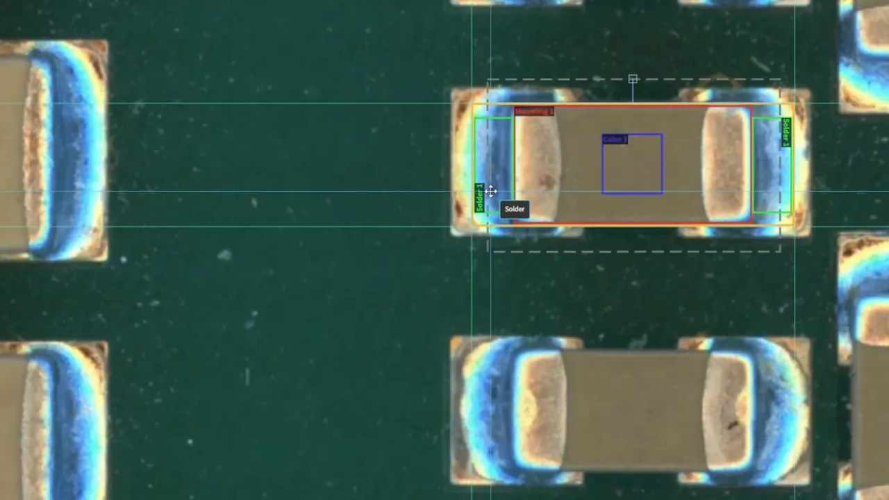
Ask an inspection engineer how many defect types a line has and the answer is usually twenty or thirty; ask how many new ones appeared last year and there are still three to five. Defect morphology has no boundary — new processes, new incoming material and new batches all bring new ways to fail. Good parts are different: a component's normal appearance does have a boundary, and that is what makes few-shot self-training possible.

ACI in this article stands for Automated Cognitive Inspection — the next-generation term for AI AOI: keep the A and the I, and replace the O (optical) with C (cognitive), because the decision basis is cognition rather than the imaging method. The full argument is set out in From AI AOI to ACI.

1. Why the defect-library route narrows over time

Rule-based and early learning-based inspection both start from a defect library: collect the known failure modes, label them, and let the model learn to recognise them. That works where defect types are stable, volumes are large and the product does not change. The difficulty sits in the word known — it only covers what you have already seen.

The more practical difficulty is cold start: a new line has the fewest defect samples exactly when inspection is most needed. To reach a workable dataset, teams either manufacture defective parts deliberately or run manual full inspection for weeks to collect them. The former produces defects that may not resemble real process failures; the latter pushes go-live back by weeks.

2. Open sets and closed sets

One level of abstraction makes it clear: the set of defects is open — you cannot enumerate it; the set of good parts is closed — a component's normal appearance is constrained by design and process and has a definite boundary.

Classifying on an open set means the model learns the failures it has seen, with no guarantee for the ones it has not. Modelling on a closed set means the model learns what normal looks like, and anything departing from normal falls on the anomaly side without having to be seen first. These are different problems with different difficulty — the second converges, the first does not.

This reversal is one of the reasons for renaming AOI as ACI; further reading: From AI AOI to ACI.

Enumerating failure modes is a task without an end. Describing what right looks like has one.

3. Three things change at once

• Cold start: no waiting for defects to accumulate. One good sample completes modelling, so a new line can inspect from day one.
• Changeover: a new model number needs no fresh defect data, because what has to be described is the new part's normal appearance — and that sample is on hand.
• Long-tail defects: a failure mode occurring for the first time does not need to have been seen before; it only has to depart from normal. This is the hardest gap for the defect-library route to close.

All three change the same underlying thing: the criterion no longer depends on how many failure modes have been seen, but on how accurately good has been described.

4. Does that remove the need for defect annotation?

No. Modelling from good parts answers “this is anomalous”, while the line still needs “which kind of anomaly” for severity, classification and process traceability. What changes is where and how much annotation happens: from “thousands of defect images before go-live” to “add categories as defects actually occur after go-live”.

The value of that order is that what gets annotated is a defect that really happened, rather than one manufactured to fill a dataset. The annotation effort also shifts from one large up-front investment to a small ongoing one that follows the line's own rhythm.

5. Which good samples to choose

Few-shot does not mean any sample will do. A few rules of thumb:

• Take parts from a stable process window, not from machine setup — a “good” part made during setup still carries an unconverged process signature.
• Cover normal variation within tolerance: colour differences between incoming batches and in-tolerance positional shift should appear in the good set, otherwise the model will treat them as anomalies.
• Do not mix in parts under dispute: if acceptance is contested, let process engineering rule on it first; until then it stays out of the good set.

These determine how accurately the boundary of normal is drawn. Draw it wrong and every later judgement inherits the error — this is the step on the few-shot route that most needs human involvement, and the only one that does.

6. How this relates to the decision layer

Modelling from good parts changes how the model learns; the decision layer changes what the criterion hangs on. The two go together: only when the criterion reads “is this component within its normal range of appearance” is the output of good-sample modelling directly usable. If the criterion is still “pixel difference from a reference image”, good-sample modelling merely yields a better reference image, and the old sensitivity to illumination and batch remains untouched.

7. When modelling from good parts is not enough

The cases where it does not apply deserve the same clarity:

• Defect and good part are indistinguishable under the imaging method in use — an internal void simply does not form an image under visible light. That is an imaging problem, not a modelling one.
• Normal appearance has not converged: during pilot production the process changes daily, so “what counts as normal” is not yet defined and modelling would lock in a wrong baseline.
• Severity depends on context rather than appearance: whether some defects are rejected depends on location, customer or batch destination. That part needs rules; a model cannot supply it.

The first two mean “not yet”; the third means “rules are needed alongside the model”. None of them argues against good-sample modelling, but together they determine how much of a given line it can cover.

8. A workable order for migrating from a defect library

A line with years of defect library behind it need not discard it. A workable order is to run both in parallel for a period:

• Step one: build a model from the good set and run it alongside the existing defect-library model. Neither drives a stop action; only the differences in judgement are recorded.
• Step two: attribute every difference. Which ones are over-calls by the good-sample model (normal variation the good set failed to cover), and which are escapes by the defect-library model (failure modes it had never seen)? The list this produces is more persuasive than any metric.
• Step three: extend the good set according to that attribution, rather than extending the defect library. Re-run the comparison until the over-calls converge.
• Step four: hand over primary responsibility for the decision, and repurpose the defect-library model for severity and classification — it remains useful for “which kind of defect”, it simply no longer answers “is there one”.

The pivotal step is the second: a difference list makes the boundary between the two routes visible, instead of deciding by whose accuracy number reads better.

9. How to tell the good set's boundary is drawn correctly

Whether the boundary is right cannot be answered by the model's own confidence — that is self-attestation. Three usable criteria exist, all of them outside the model:

• Cross-batch consistency: model on batch A's good parts and run batch B's good parts through it. If batch B is flagged heavily, the good set failed to cover between-batch normal variation and the boundary is drawn too tight.
• Review overturn rate: the share of model-flagged anomalies that human review overturns, aggregated by component type. Concentrated overturns for one component type mean that part's normal appearance is under-described.
• Where disputed parts land: keep parts that process engineering has ruled acceptable in a separate group, out of the good set, and run them after modelling. Their verdicts show directly which side of the boundary they fall on.

What the three share is that the criterion rests on facts outside the model — another batch's good parts, a human review conclusion, a process ruling. Using the model's own output to prove the model right is the easiest mistake to make on this route.

Decoupling the decision layer from the imaging method is the other half of the same route; see More than one imaging method on a line.

Full solution for this scenario: the full inspection solution for AI AOI Software

This article was generated by AI. Customer cases are simulated scenarios based on real product capabilities and figures are illustrative; see product pages for official benchmarks.